OpendTect Fault Mapping in Time Slices

Version: OpendTect 6.0

We generally think about mapping faults in vertical seismic sections because the fault offset is visible and we are used to this view from outcrop work. However, in terrain with complex faulting this approach is limited. For example, it may be that faults are oblique to both the inline (IL) and cross line (XL) directions, are strike-slip or oblique-slip with little or no vertical throw and therefore would be undetectable on in the vertical view, or the fault network is very complex and difficult to unravel from vertical sections.

A 3D seismic fault mapping workflow in these difficult situations for OpendTect 6.0 is given below. The example is from the Vermillion area offshore Louisiana in the Gulf of Mexico (data credit: FairfieldNodal). This data has bin size 55x55 ft and time sample rate of 6 ms.

1. Identify the fault block (FB) to be mapped using IL and XL seismic amplitude sections (Fig 1).
2. Open a time slice (TS) at the FB level displaying seismic amplitude PSTM data (Fig 2). Although major faults will likely be visible in the amplitude data, subtle faults will be overlooked if we interpret faults on this data type. 
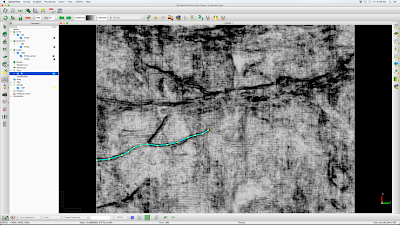
1. The fault mapping attribute we want to use is similarity. In this example a similarity data cube has been computed with vertical window of +/- 48 ms.  Long-window similarity provides a good image of faults that are nearly vertical over the extent of the time window (~100 ms in this case). Display similarity in the TS to reveal a much better view of the fault network (Fig 3).
3. Set the time slice step to 60 ms and move TS up above the block of interest, but be sure the faults of interest are still present (Fig 4). 
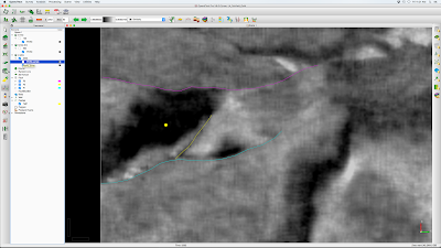
4. Create a new fault and save as F1, set color to Cyan. In the TS, click along the fault (Fig 5). Step down TS by 60 ms picking this fault in each slice. As with horizons, the 'v' key toggles between 'show in full' and show the fault only in the working TS. In the example, this process allows construction of the fault from 1960-2500 ms (Fig 6, Fig 7). Note that in the vertical view the constructed fault shows an un-geologic zig-zag pattern related to the window length of the similarity attribute used. Picking faults directly in vertical sections can be done in simpler areas to yield a more geologically reasonable fault line, but the method given here is good enough in complex areas.
5. Create new fault and save as F2, set color to yellow. Repeat as above on cross fault.
6. Create new fault and save as F3, set color to magenta. Repeat as above on N fault.
7. This process maps all faults around the block of interest as seen on similarity (Fig 8) and PSTM (Fig 9). A 3D view is given in Fig 10.

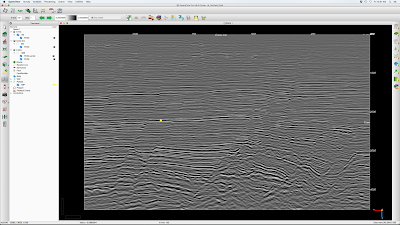Fig 1. PSTM inline section with yellow pick point on fault block to be mapped. 

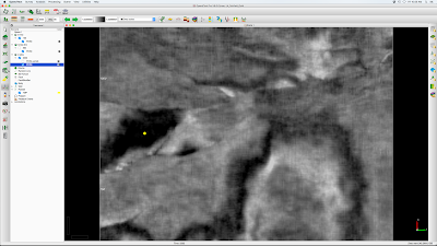Fig 2. Time slice through PSTM data at pick point level.

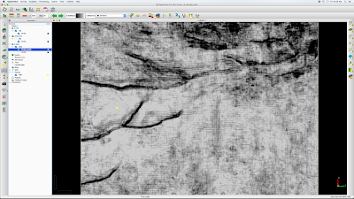Fig 3. Similarity data gives a much better map view of faults.

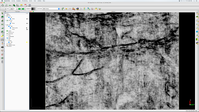Fig 4. Similarity TS above the horizon of interest.

Fig 5. Fault F1 created and picked in shallow TS.

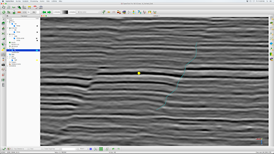Fig 6. IL view of horizon and F1 fault shown only in section.

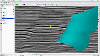Fig 7. IL view of horizon and F1 fault shown in full.

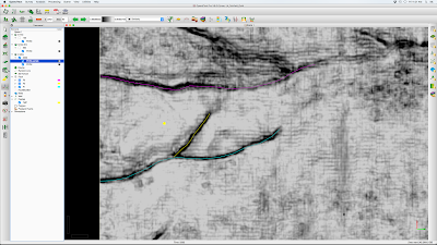Fig 8. Repeating the process for faults F2 (yellow) and F3 (magenta), surrounds the block of interest.

Fig 9. All faults shown on PSTM data. It would not have been possible to pick faults to this accuracy on PSTM data alone.

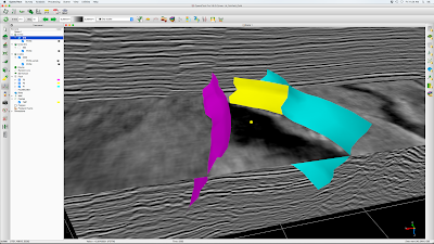Fig 10. 3D view of TS, IL, event pick and faults surrounding the block of interest.